R's nrow and ncol considered harmful
1 June 2013I've recently had to compare various bias/variance/time-efficiency properties of a set of statistical estimators to see which would be the preferred method of estimation in certain circumstances. While formerly this task would have been done in MATLAB, I've been making an effort lately to port my work to R, mostly out of respect for open-sourcedness and portability but also because the graphs it makes are light years ahead of MATLAB's plots (while its plotting facilities have a steeper learning curve they have a far sweeter payoff once the initial hump is crossed).
My code was running somewhat slowly, so I started checking for bottlenecks; I was certain that the fault would lie in eigen, chol, solve or some other matrix method. I was quite wrong. For the purposes of one of the estimators, it is necessary to construct a set of new matrices of sizes corresponding to various parameters in the model; these parameters happen to be related to the size of input data matrices, so rather than pass them around willy-nilly the script was computing them from the properties of the matrix.
To determine the size of a matrix, R provides the useful functions nrow and ncol, which do about what you'd expect them to do. And it turns out these functions do this quite slowly. R provides another dimension-checking function, dim which returns an array of the size of the matrix along various dimensions. In this sense, given a matrix A, we have (in the loose sense)
nrow(A) == dim(A)[1]; # TRUE
ncol(A) == dim(A)[2]; # TRUE
So the results are reasonable and the methods are identical. Given the notational overhead and the fact that nrow and ncol should have access to the same data as dim (assuming dimensions are stored as part of the object, or are computed only as needed), it is extremely counterintuitive that they should run more slowly. But they do.
The code we use to test this is as follows:
rowcoltest = function ( M, R )
{
  tdim = 1 : R;
  trc  = 1 : R;
  m    = 0;
  n    = 0;

  for ( r in 1 : ceiling( R / 2 ) )
  {
    t0     = proc.time()[3];
    m      = nrow( M );
    n      = ncol( M );
    trc[r] = proc.time()[3] - t0;

    t0      = proc.time()[3];
    d       = dim( M );
    m       = d[1];
    n       = d[2];
    tdim[r] = proc.time()[3] - t0;
  }

  for ( r in ( ceiling( R / 2 ) + 1 ) : R )
  {
    t0      = proc.time()[3];
    d       = dim( M );
    m       = d[1];
    n       = d[2];
    tdim[r] = proc.time()[3] - t0;

    t0     = proc.time()[3];
    m      = nrow( M );
    n      = ncol( M );
    trc[r] = proc.time()[3] - t0;
  }

  return( list( tdim = tdim, trc = trc ) );
};

testmaster = function ( ms, ns, R )
{
  results = list();

  for ( m in ms )
  {
    for ( n in ns )
    {
      M = matrix( rnorm( m * n ), nrow = m );
      T = rowcoltest( M, R );

      results[[ length( results ) + 1 ]] = list(
        m = m,
        n = n,
        T = T
      );
    }
  }

  return( results );
}

resultstodf = function ( results )
{
  ms = c();
  ns = c();
  trc = c();
  tdim = c();

  for ( i in 1 : length( results ) )
  {
    ms   = c( ms, results[[i]]$m );
    ns   = c( ns, results[[i]]$n );
    trc  = c( trc, sum( results[[i]]$T$trc ) );
    tdim = c( tdim, sum( results[[i]]$T$tdim ) );
  }

  results_df = data.frame( m = ms, n = ns, rowcol = trc, dim = tdim );
}

R  = 100000;
ms = c( 1, 10, 100, 1000 );
ns = c( 1, 10, 100, 1000 );

T   = testmaster( ms, ns, R );
Tdf = resultstodf( T );
print( Tdf );

sum( Tdf$rowcol ) / sum( Tdf$dim );
mean( Tdf$rowcol / Tdf$dim );
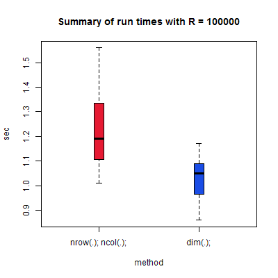
Simple enough: construct a timing harness to discover the run-time of the two methods of determining array size, then run it R = 100000 times. The results are as follows:
> print( Tdf );
      m    n rowcol  dim
1     1    1   1.22 0.94
2     1   10   1.01 1.17
3     1  100   1.05 1.08
4     1 1000   1.38 0.98
5    10    1   1.48 1.03
6    10   10   1.12 1.15
7    10  100   1.10 1.09
8    10 1000   1.11 1.07
9   100    1   1.16 0.86
10  100   10   1.44 1.09
11  100  100   1.22 1.08
12  100 1000   1.56 1.00
13 1000    1   1.22 1.00
14 1000   10   1.29 1.15
15 1000  100   1.14 0.89
16 1000 1000   1.05 0.95
>
> sum( Tdf$rowcol ) / sum( Tdf$dim );
[1] 1.182698
> mean( Tdf$rowcol / Tdf$dim );
[1] 1.192896
Depending on how you measure, to a first approximation it's safe to say that using a combination of nrow and ncol is 20% slower than using dim and dereferencing the results! Obviously this is for only a single run (of \( R=100000 \)), but this result holds up across operating systems — tested on Windows, Ubuntu, and whatever Unix our cluster runs — and more or less across time and other uses of my CPU, though the approximation is reduced to nrow and ncol being 15% worse.
Moral of the story: if you want to dynamically determine the size of your input matrices in R (it's not clear if this applies to anything other than matrices) and have to do so more than a few times, use dim to determine the size of all dimensions, then dereference the result.
why is this?
This post sat in my “finish eventually” queue for over two years. In that time I've learned to be somewhat more suspect regarding empirical results like this; surely there's a reason that dim is faster!
Investigating, it's obvious:
> nrow
function (x)
dim(x)[1L]
<bytecode: 00000000057EEA58>
<environment: namespace:base>
> ncol
function (x)
dim(x)[2L]
<bytecode: 00000000062CF0B0>
<environment: namespace:base>
> dim
function (x)  .Primitive("dim")
That is, dim is a primitive, while nrow and ncol are aliases (essentially) for calling-and-dereferencing dim. The reason for slowness is therefore pretty straightforward: using nrow and ncol to determine the size of both dimensions of a matrix requires two calls to dim, while dim requires only one. Knowing what's going on under the hood, we can reinterpret our results.
New moral of the story: for clarity of code, it is safe to use nrow or ncol to determine the size of one dimension of a matrix; if you need to determine two or more dimensions, use dim instead.
Included \(\LaTeX\) graphics are generated at LaTeX to png or by ![]() .
.
contemporary entries
- "dynamic" dns updates for 1&1 hosting (30 August 2013)
- reaction (5 June 2013)
- R's nrow and ncol considered harmful (1 June 2013)
- tools for tas (19 May 2013)
- on white elephant (5 May 2013)
view all entries »
comments
there are no comments on this post